


This is a collection of graphical demonstrations of concepts in complex analysis which I developed for a course I gave on that subject during the spring semester of 1997. (For graphical demonstrations of calculus concepts see my page on Graphics for the calculus classroom.)
If your browser supports Java, the latest version of this page is preferable to this one. There is also a version based on animated GIFs. These later versions have more and better quality graphics.
The most common method of visualizing a complex map is to show the image under the map of a set of curves, e.g., a set of line segments of constant real and/or imaginary part (a Cartesian grid), or a set of concentric circles and spokes (a polar grid). A weakness of this approach is that it can be difficult or impossible to infer which points of the original curves are mapped to which points of the final images. The graphics on this page use two techniques to overcome this problem. First, most are animated so that the original curves are continuously deformed into the image curves, and the eye can follow which points move where. Second, I use colors to distinguish different points and curves.
The animations on this page are in FLI/FLC format. Viewers for this format are available for most platforms. You'll get the most from the animations by controlling the frame advance manually (which is possible with most viewers). If you can't control the frame advance manually, it is best to put the viewer in shuttle, or ping-pong, mode and adjust the frame advance speed to rather slow.
The squaring mapAs a first example, consider the simple function
![]() .
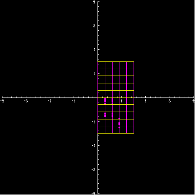
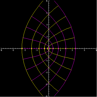
We shall examine how a square with corners at
.
We shall examine how a square with corners at
![]() is transformed under this map. First we just look at the half of the square
in the right half plane, which is shown in the first
frame (3K).This region mapped one-to-one onto
the region contained between two parabolas, exhibited in final
frame (5K).The lines of constant real part are
mapped onto parabolas opening along the negative real axis, and those with
constant imaginary part to parabolas opening along the positive real axis.
Note that these parabolas meet at right angles, a consequence of conformality
(see below). The frames of the animation
(196K) show the image of the half-square under a linear
combination of the identity map and the squaring map:
is transformed under this map. First we just look at the half of the square
in the right half plane, which is shown in the first
frame (3K).This region mapped one-to-one onto
the region contained between two parabolas, exhibited in final
frame (5K).The lines of constant real part are
mapped onto parabolas opening along the negative real axis, and those with
constant imaginary part to parabolas opening along the positive real axis.
Note that these parabolas meet at right angles, a consequence of conformality
(see below). The frames of the animation
(196K) show the image of the half-square under a linear
combination of the identity map and the squaring map:
![]() ,
with t increasing from 0 to 1. In other word, this is an animation of the
linear homotopy taking the identity to the squaring map. Note that the
intermediate maps are again quadratic in z and hence conformal at
all but one point.
,
with t increasing from 0 to 1. In other word, this is an animation of the
linear homotopy taking the identity to the squaring map. Note that the
intermediate maps are again quadratic in z and hence conformal at
all but one point.
The next animation (148K) shows the deformation of the half of the square lying in the left half plane. This region is mapped one-to-one onto the same region and the right half of the square. Therefore the deformation of the entire square (251K) shows the square being folded over onto itself as it distorts, so as to cover the parabolically bounded region twice. If you pause the animation on the penultimate frame, the two-to-one character of the map is evident.
The squaring map behaves more simply when applied to a polar grid, since it takes circles of constant modulus to circles of constant modulus, and rays of constant argument to rays of constant argument. We animate the deformation of the disc of radius 2 centered at the origin and overlayed with a polar grid. The animations show the deformation of the half disc in the right half plane (215K), the deformation of the half disc in the left half plane (174K), and the deformation of the entire disc (316K).
A better view of the same map comes when the disc is colored, here by a hue which varies with the argument (so the color is constant on each ray emanating from the origin). An animation of the colored disc (536K), displays clearly how the disc is folded over on itself to cover the image disc twice (again, pause a few frames from the end). The discontinuity in the coloring in the final frame reflect the impossibility of defining a continuous square root function on the disc. By looking at the last few frames, it is also possible to get a pretty clear idea of the Riemann surface for the squaring map (a surface which, when realized in 3 dimensional space, intersects itself along the negative real axis).
The exponential, sine, and cosineThe same techniques of visualization apply to other complex maps. For
example, the complex exponential (505K)
maps the infinite open strip bounded by the horizontal lines through
![]() one-to-one onto the plane minus the negative real axis. The lines of constant
real part are mapped to circles, and lines of constant imaginary part to
rays from the origin. In the animation we view a rectangle in the strip
rather than the entire strip, so the region covered is an annulus minus
the negative real axis. The inner boundary of the annulus is so close to
the origin as to be barely visible. We also make the strip a bit thinner
than
one-to-one onto the plane minus the negative real axis. The lines of constant
real part are mapped to circles, and lines of constant imaginary part to
rays from the origin. In the animation we view a rectangle in the strip
rather than the entire strip, so the region covered is an annulus minus
the negative real axis. The inner boundary of the annulus is so close to
the origin as to be barely visible. We also make the strip a bit thinner
than ![]() ,
so that the annulus does not quite close up.
,
so that the annulus does not quite close up.
The next animations show two-to-one coverings of a disc by the complex cosine (653K) and complex sine (655K) restricted to suitable rectangles.
ConformalityAn important property of analytic functions is that they are conformal
maps everywhere they are defined, except where the derivative vanishes.
A conformal map is one that preserves angles. More precisely, if two curves
meet at a point and their tangents make a certain angle there, then the
angle between the images curves under any analytic function (with non-vanishing
derivative) will be the same in both sense and magnitude. A consequence
of conformality, namely the preservation of orthogonality of intersecting
coordinate lines, was visible in all the animations above. Another nice
example is given by the power map (138K)
![]() ,
which is conformal everywhere except at the origin. Here we apply the map
to a square grid in the first quadrant, with the power a varying from 1
to 3.9. Notice how all the right angle intersections remain right angles
throughout the deformation, except the angle made by the green lines meeting
at the origin, where the power maps are not conformal.
,
which is conformal everywhere except at the origin. Here we apply the map
to a square grid in the first quadrant, with the power a varying from 1
to 3.9. Notice how all the right angle intersections remain right angles
throughout the deformation, except the angle made by the green lines meeting
at the origin, where the power maps are not conformal.
My favorite demonstration of conformality is to view the deformation
of four small squares (58K) under a cubic polynomial
in the complex variable z (namely
![]() ).
Notice that the squares deform only by dilating
and rotating. This is another way to express conformity. By contrast, if
we replace the quadratic term of the polynomial by its conjugate
(so
).
Notice that the squares deform only by dilating
and rotating. This is another way to express conformity. By contrast, if
we replace the quadratic term of the polynomial by its conjugate
(so ![]() ),
we get
another cubic polynomial map, but this one is not analytic, and clearly
not conformal (46K). Note also, that conformality
is a local property. If we think of the four small squares as the vertices
of a larger square, that square is vastly deformed, not just dilated and
rotated.
),
we get
another cubic polynomial map, but this one is not analytic, and clearly
not conformal (46K). Note also, that conformality
is a local property. If we think of the four small squares as the vertices
of a larger square, that square is vastly deformed, not just dilated and
rotated.
M�bius TransformationsM�bius transformations are widely studied as a useful example of conformal maps. A key property is that they map circles in the Riemann sphere into circles in the Riemann sphere, or, equivalently, that the image of a line or circle in the plane is another line or circle. This animation (1M) shows the identity map (a M�bius transformation!) being deformed into a less trivial M�bius transformation. The homotopy is chosen so that all the intermediate steps are M�bius transformations as well. The animation shows the unit square deformed into a closed curve composed of four circular arcs. The inside of the square is mapped to the region outside of the curve, and a region about infinity is mapped to the interior of the curve. The specific family of M�bius transformations displayed is
![]()
How were these graphics made?Finally, for those interested in the technical details, or perhaps for making graphics of one's own, you can see how these graphics were made.
 This
work is licensed under a
Creative Commons Attribution-Noncommercial-Share Alike 3.0 License.
This
work is licensed under a
Creative Commons Attribution-Noncommercial-Share Alike 3.0 License.