
10x20 mesh of the unit square
Douglas N. Arnold 2014
As a first problem we consider the Neumann boundary value problem: \[\tag{1} -\Delta u + u = f \text{ in $\Omega$}, \quad \frac{\partial u}{\partial n} = 0 \text{ on $\partial\Omega$}, \] where \(\Omega\) is a domain in \(\mathbb R^2\). This problem is particularly simple in that it does not involve coefficient functions or essential boundary conditions, and the natural boundary conditions are homogeneous. We will get to those aspects soon enough, but its nice to ignore them the first time through. Notice that we do include a zero degree term in the PDE (\(-\Delta u + u\) rather than just \(-\Delta u\)), since otherwise the Neumann problem would not be well-posed: any constant function would solve the problem for \(f=0\).
As always for finite elements, we will solve the problem in weak form. Thus we seek a function \(u\) in a trial space \(V\) such that \[b(u,v) = F(v) \qquad \text{for all test functions $v\in V$}. \] For the boundary value problem (\(1\)) the trial space \(V=H^1(\Omega)\), and the bilinear form \(b:V\times V\to \mathbb R\) and the linear functional \(F:V\to \mathbb R\) are given by \[ b(u,v)= \int_\Omega (\operatorname{grad}u\cdot\operatorname{grad}v + uv)\,dx, \quad F(v) = \int_\Omega fv\,dx. \]
A test problem. To specify a test problem, we start with the solution \(u(x,y) = [(x^2-2x)\sin 2\pi y]^2\) on the unit square \(\Omega=(0,1)\times(0,1)\). This function satisfies the homogeneous Neumann boundary conditions, so we take \(f=-\Delta u + u\), and then \(u\) is indeed the exact solution of \((1)\). By direct calculation we find that \[ \begin{align*} \tag{2} f(x,y) &= -8[\pi(x^2-2x)]^2\cos 4\pi y \\ &+ (x^4-4x^3-8x^2+24x-8)\sin^2 2\pi y. \end{align*} \]
The finite element solution \(u_h\in V_h\) is then determined from the Galerkin equations \[ b(u_h,v) = F(v), \quad v\in V_h, \] where \(V_h\) is the finite element subspace we use to approximate \(V\). We shall take \(V_h\) to be the Lagrange space of degree 2, which means that we choose a mesh (triangulation) of the domain \(\Omega\), and that \(V_h\) consists of all continuous functions on \(\Omega\) which restrict to polynomials of degree at most 2 on each triangle of the triangulation.
Specifying the mesh. Before turning to the FEniCS implementation, we discuss how the data of the problem is expressed in FEniCS. In this case, the only data we need to supply is the mesh (which implies the domain), and right-hand side function \(f:\Omega\to\mathbb R\). There are numerous ways to define a mesh in FEniCS. It may be constructed externally to FEniCS by various different programs, then written to a file in an appropriate format and imported into FEniCS. Alternatively, there are several ways to construct a mesh inside FEniCS. Some of these require that FEniCS was compiled with a package known as CGAL, which may or may not be the case depending on the particular FEniCS installation. We shall use the FEniCS function UnitSquareMesh which constructs a structured mesh of the unit square and is present in all FEniCS installations. Specifically, the code
mesh = UnitSquareMesh(10, 20)produces the mesh obtained by dividing the unit square into \(10\times 20\) rectangles and dividing each of these into two triangles with the positively sloped diagonal, yielding this mesh of 400 elements:
10x20 mesh of the unit square
Specifying the right-hand side. In order to define the functional \(F(v)=\int_\Omega fv\,dx\) we have to specify the function \(f\) on \(\Omega\). The simplest way to do this is define a FEniCS Expression, which translates the expression \((2)\) for \(f\) in terms in the coordinates of the point. The coordinates are expressed as \(x[0]\) and \(x[1]\), rather than \(x\) and \(y\) as used in \((2)\). To the occasional surprise of FEniCS novices, the expressions must be given in a string that will be parsed by a C++ compiler. These usually look pretty identical to python expressions and math expressions in other languages, but one exception is that exponentiation \(a^b\) must obtained through the pow function: pow(a, b). Taking this into account, we get the following line of code to define \(f\).
f = Expression('-8 * pow(pi*(pow(x[0], 2) - 2*x[0]), 2) * cos(4*pi*x[1]) \
      + (pow(x[0], 4) - 4*pow(x[0], 3) - 8*pow(x[0], 2) + 24*x[0] - 8) \
        * pow(sin(2*pi*x[1]), 2)')
We are now ready to present the full FEniCS implementation. As you can see, it is just 10 python statements, and it follows the mathematical specification of the discrete problem closely.
from dolfin import *  # import FEniCS into python
# define the function f
f = Expression('-8 * pow(pi*(pow(x[0], 2) - 2*x[0]), 2) * cos(4*pi*x[1]) \
      + (pow(x[0], 4) - 4*pow(x[0], 3) - 8*pow(x[0], 2) + 24*x[0] - 8) \
        * pow(sin(2*pi*x[1]), 2)')
# define the mesh and the function space
mesh = UnitSquareMesh(10, 20)
Vh = FunctionSpace(mesh, 'Lagrange', 2)
# define the bilinear form b(u, v) and the linear function F(v)
# for any trial function u in V_h, test function v in V_h
u = TrialFunction(Vh)
v = TestFunction(Vh)
b = (dot(grad(u), grad(v)) + u*v)*dx
F = f*v*dx
# solve the Galerkin equations for the function u_h in V_h
uh = Function(Vh) # this declares u_h as finite element function in V_h
solve(b == F, uh)
At this point uh is the finite element solution. We can use it in various ways. For example we can plot it using the the basic plotting capability built into FEniCS:
plot(uh) # use plot(uh, interactive=True) to manipulate the plot
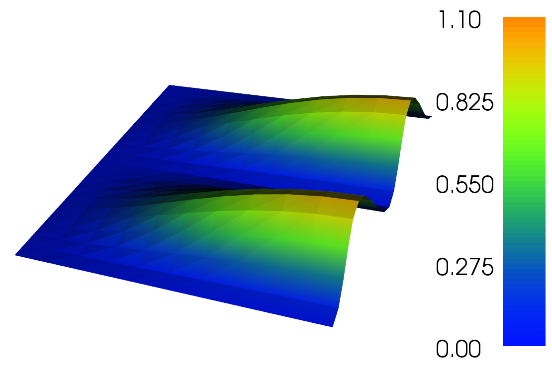
Finite element solution
For more advanced plotting, one can export the solution to a PVD file, which can be imported to the ParaView visualization program for plotting:
File("solution.pvd") << uh

ParaView plot of solution
We can simply evaluate the computed solution at a point. At the point \((3/4, 3/4)\), the exact solution is \(u(3/4,3/4)=225/256 = 0.87890625\). Compare with evaluation of the computed solution:
value = uh(0.75, 0.75)
exact = 225./256.
error = (exact - value)/exact
print "value at (3/4, 3/4): {:10.8f},  error = {:6.4f}%".format(value, 100*error)
Since uh is a finite element function, we can act on it in various ways. For example, we can compute its integral over \(\Omega\) using finite element assembly. Compare with the exact value which is \(4/15=0.2666\ldots\):
uhint = assemble(uh*dx)
exact = 4./15.
error = (exact - uhint)/exact
print "integral of solution: {:10.8f},  error = {:6.4f}%".format(uhint, 100*error)
Suppose that our PDE were \[
-\operatorname{div}(a\operatorname{grad}u) + c u =f
\] instead of just \(-\Delta u+u = f\), now involving variable coefficients \(a,c:\Omega\to\mathbb R\). Thus the bilinear form would become \[
b(u, v) =\int_\Omega (a\operatorname{grad}u\cdot\operatorname{grad}v+cuv)\,dx+\cdots
\] It is not hard to imagine how this would be entered in FEniCS. Each of the coefficients \(a\), and \(c\) would be defined as an Expression, just as \(f\) was above, and then these expressions would enter the definition of the bilinear form, which would mimic closely the equation above:
b = (a*dot(grad(u), grad(v)) + c*u*v)*dxVector, matrix, and higher order tensor coefficients are allowed as well as, for example, in the following code:
A = Expression((('2.', '.5*x[0]'), ('.5*x[0]', '4. + x[0]*x[1]')) # matrix coefficient
b = dot( dot(A, grad(u)), grad(v))*dxSo what is happening when we run the above program? From the statement
Vh = FunctionSpace(mesh, 'Lagrange', 2)FEniCS knows the nature of finite element functions in this space. In particular it can compute the local and global degrees of freedom, one for each vertex and edge midpoint, and the corresponding basis functions \(\phi_i\). When we create an element in this space, with the statement uh = Function(Vh) it creates a vector whose length is the number of DOFs, and when we solve the finite element system with the statement
solve(b == F, uh)it computes the entries of that vector, namely the coefficients \(\alpha_j\) in the basis expansion \[
u_h = \sum_{j=1}^{\#DOFs} \alpha_j\phi_j.
\] Later when we operate on \(u_h\), every operation must be carried out by acting on the vector \(\alpha_j\) and using knowledge of the basis functions. For example, when we invoke uh(0.75, 0.75) FEniCS locates the triangle in the mesh containing the point, thereby determining which 6 of the \(\phi_j\) are nonzero there, evaluates these basis functions at the point, multiplies their values by the corresponding 6 coefficients \(\alpha_j\), and adds the products together to get the result.
The solve statement is where most of the work is concentrated. It combines several steps. First, the stiffness matrix associated to the bilinear form \(b\) is assembled. This results in a sparse matrix \(B_{ij}\) with entries \(b(\phi_j,\phi_i)\), stored only if the \(i\)th and \(j\)th DOF belong to a common triangle (otherwise \(B_{ij}=0\) and need not be computed or stored). By default FEniCS uses the PETSc toolkit for linear algebra, a highly tuned suite of datastructures and routines for working with sparse matrices. Next FEniCS assembles the load vector associated to \(F\). Then FEniCS calls PETSc routines to solve the matrix equation and determine the coefficient vector. By default a sparse direct solver is used, but this can be changed to use any of a large number of iterative solvers. Although the assembly and other operations add overhead, for large problems, the time to solve the matrix equations is almost always the dominant cost of a finite element computation.
The solve command is convenient. But is also possible to carry out the steps separately. For example, the command B=assemble(b) would create the stiffness matrix stored as a sparse matrix.
# this cell is present to set the notebook style
from IPython.core.display import HTML
def css_styling():
    styles = open("../styles/dna1.css", "r").read()
    return HTML(styles)
css_styling()