Math 5421 Spring 2025
Introduction to Climate Models

Assignment 1
due January 23

Global Mean Temperature

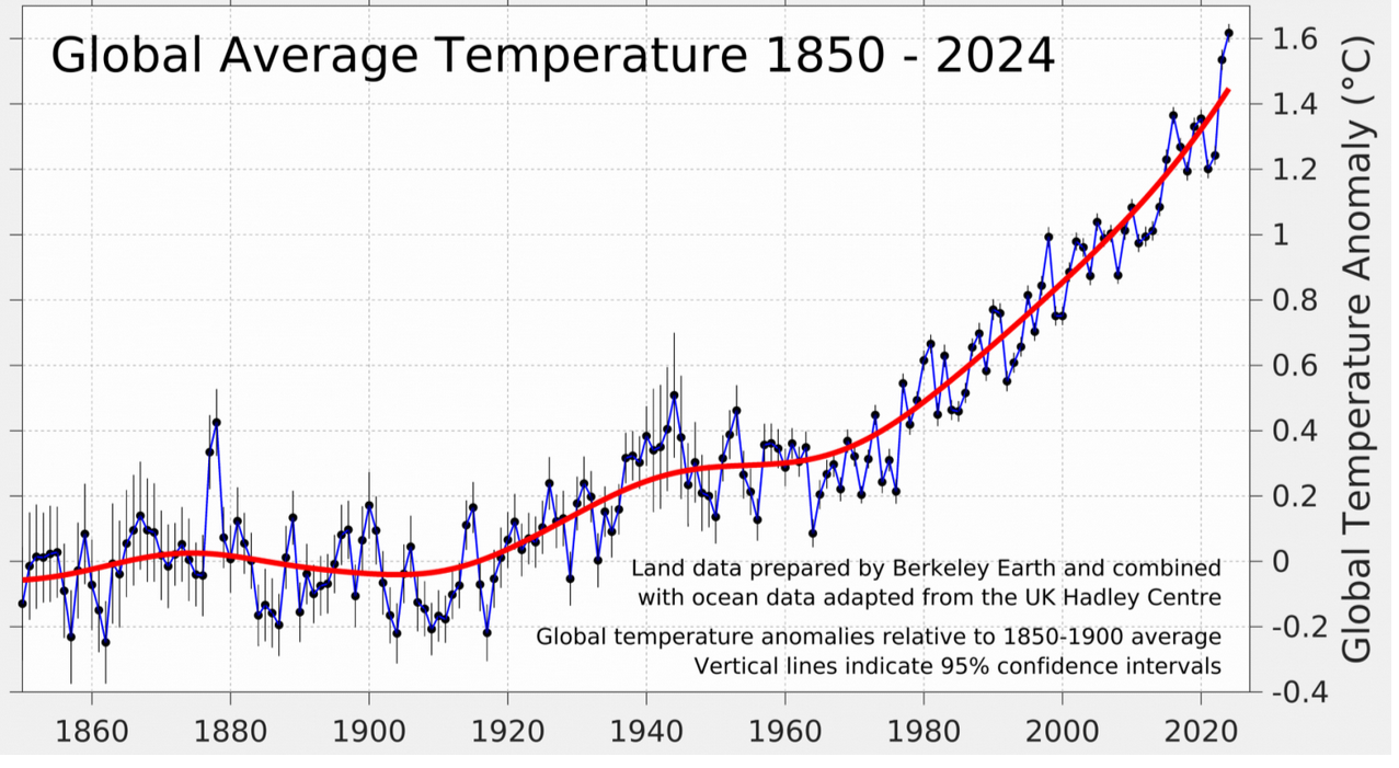There are a variety of ways to measure the surface temperature and to estimate the average over the whole Earth. For example, the National Oceanic and Atmospheric Administration (NOAA) measured the air temperature at a height of two meters above the surface, while an organization called Berkeley Earth estimates the actual surface temperaure of the land, ocean, and ice. For this workshop, we arbitrarily will use the Berkeley Earth data, a graph of which is shown in the figure on the left.

The data are available for download from Berkeley Earth at this link:

https://berkeleyearth.org/data/.

However, the data are monthly and the anomaly is measured from a different base temperature than the pre-industrial average, so I have adjusted the data to conform to the standard of setting zero to be the average global mean temperature between 1850 and 1899. Also, I have transformed the data from monthly to yearly. The link for this data set is:

https://www-users.cse.umn.edu/~mcgehee/Course/Math5421/data/BEarthGMTYearly.csv

Exercise 1

Download the data from the link given above and produce a graph like this:

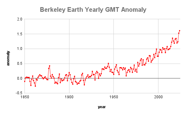
Make your graph available on Google Sheets and share it with mcgehee@umn.edu.

Twenty-first Century

For now we will focus on the 21st century, since that is the period in which we are living. Here is a link to the Berkeley Earth monthly data restricted to the 21st century:

https://www-users.cse.umn.edu/~mcgehee/Course/Math5421/data/BEarthGMTMonthly_21.csv

Note that the first three columns all contain date information. The first column is the year, the second is the month, and the third is the date expressed as the year plus the fractional part of the year from 0:00 am on January first to 12:00 pm on the fifteenth of the month. For example, the decimals 0.0411 in 2000.0411 mean that the middle of January occurs 411/1000 of the way through the calendar year. It is the third column that is useful for making graphs as a function of the date. The fourth column is the temperature anomaly in Celsius, normalized so that the average anomaly from 1850 to 1899 is zero.

Exercise 2

Download the data from the previous link and produce a graph like this:

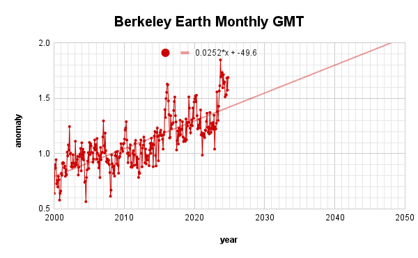
Be sure to include the "trendline" in your figure. Assuming that the trend continues through the first half of this century, when do you expect the anomaly to reach 1.5? When do you expect it to reach 2.0?

Indicate your answers on your graph, make it available on Google Sheets, and share it with mcgehee@umn.edu.