Math 5421 Spring 2025
Introduction to Climate Models

Assignment 3 Solutions

Exercise 1

Using the data in the file linked below, draw two figures.

https://www-users.cse.umn.edu/~mcgehee/Course/Math5421/data/Emissions_1959-2023.csv

The first should show the emissions for each year starting in 1959 and ending in 2023. The second should show the cumulative emissions for each year during that period. For example, the cumulative emissions in 2020 is the sum of the emissions for the years starting in 1959 and ending in 2000.

(a) For the first figure, use a linear trend and extend the axes out to 2050. If the trend continues, what do you expect the annual emissions to be in 2030? In 2050?

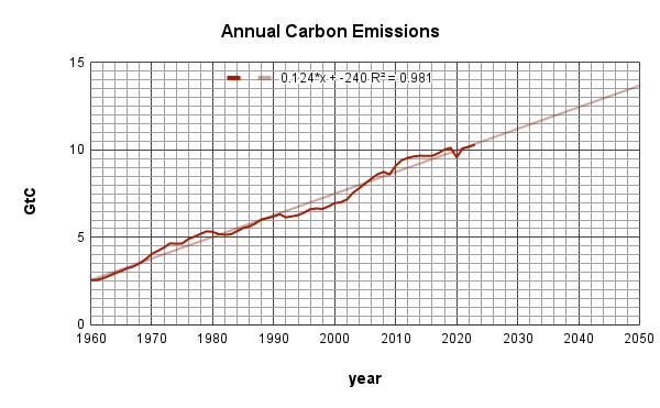
For the linear trend, we expect the annual emissions to reach about 11.2 GtC in 2030 and about 13.6 GtC in 2050.

(b) For the second figure, used a quadratic trend and extend the axes out to 2050. If the trend continues, what do you expect the cumulative emissions to be in 2030? In 2050?

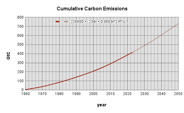
For the quadratic trend, we expect the cumulative emissions to reach about 490 GtC in 2030 and about 730 GtC in 2050.

(c) Using your knowledge of the Fundamental Theorem of Calculus, justify the use of the quadratic trend in the second figure.

Since the cumulative emission is the integral of the annual admissions, since the annual emissions fit a linear trend pretty well, and since the integral of a linear function is a quadratic function, we would expect the quadratic trend to be the appropriate fit.

Exercise 2

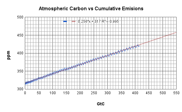
Using the data in the file linked below, produce a scatter plot with the cumulative emissions on the horizontal axis and the atmospheric CO2 on the vertical axis. Include in your figure the linear trend.

https://www-users.cse.umn.edu/~mcgehee/Course/Math5421/data/MLOCO2vsCumulEmiss.csv

(a) Ask your favorite AI whether the increase in atmospheric CO2 is caused by human activity. Report the answer, and use your figure to either support or dispute the AI's answer.

There is no right answer.

(b) Using the slope of your trend line compute the percentage of emitted CO2 that has remained in the atmosphere since 1959.

We see from the displayed equation that the slope of the trend line is 0.256, which implies that for every 100 GtC emitted, the atmospheric carbon has increased by 25.6 ppm, or 2.13×25.6 = 54.5 GtC. Therefore, the percentage of carbon remaining in the atmosphere is 54.5%.

(c) Assuming that the trend in your figure continues into the future, what will be the atmospheric CO2 if we emit another 100 GtC?

We computed in part (b) that the atmospheric concentration will increase by 25.6 ppm. The data set we are using tells us that the atmospheric concentration in December of 2023 was about 421.6 ppm while the cumulative emissions were about 415.5 GtC. We would conclude that, when the cumulative emissions reach 515.5 GtC, we expect the atmospheric concentration to be about 447 ppm.

Alternatively, we could look at the Keeling Curve Website and see that the atmospheric concentration on January 31, 2025, was 426 ppm. Therefore, an additional emission of 100 GtC from January 31, 2025, would result in an atmosphic concentration of about 452 ppm.

Exercise 3

Using the data in the file linked below, produce a scatter plot with the cumulative emissions on the horizontal axis and the GMT anomaly on the vertical axis. Include in your figure the linear trend.

https://www-users.cse.umn.edu/~mcgehee/Course/Math5421/data/AllTogetherNow.csv

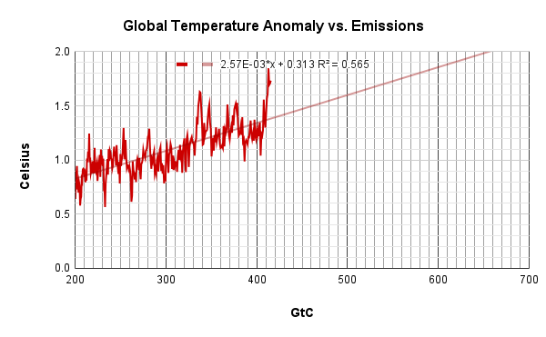
(a) Using the slope of the trendline, estimate how much more CO2 can be emitted before the temperature anomaly reaches 1.5°C. Same estimates for 1.7°C and 2.0°C.

From the trendline in the figure above, we see that the anomaly will reach 1.5°C when the cumulative emissions reach about 460 GtC. We see from the data that the cumulative emissions at the end of 2023 were about 421.6 GtC. Starting in January of 2024 we could emit an additional 460−421.6 or about 38 GtC before the temperature reached 1.5°C.

The trend line in figure also indicates that an anomaly of 1.7°C would occur if the cumulative emissions reach 5400 ppm. We would reach this anomaly if we emitted 540−421.6 or about an additional 118 GtC starting in 2024.

The trend line also indicates that an anomaly of 2.0°C would occure if the cumulative emissions reach about 655 ppm. We could reach this anomaly if we emit an additionsl 655−421.6 or about an additional 233 GtC over 2023 levels.

For the following questions, assume that, starting in 2024, you owned all the carbon emitting industries on the planet and that you have complete control of what they do.

(b) If, starting in 2024 you held all carbon emissions to 10 GtC/year, when would the GMT anomaly reach 1.5°C? When would it reach 2.0°C?

We saw in part (a) that an additional 38 GtC of emissions would result in a temperature anomaly of 1.5°C. At 10 GtC starting in 2024, we would reach 1.5°C in the fall of 2027.

We also saw that an additional 233 GtC of emissions would result in a temperature anomaly of 2.0°C. At 10 GtC per year, we would reach 2.0°C in 2047.

(c) If, starting in 2024, you held emissions to 10 GtC, then reduced the emissions by 2 GtC each year until you reached net zero in 2029. What would the temperature anomaly be in 2029?

The total additional carbon emitted would be 10+8+6+4+2=30 GtC. Using the data that the total cumulation at the end of 2023 was 421.6 GtC, an additional 30 GtC would take us to 451.6 GtC, which would be an anomaly of about 1.48°C.

(d) Same as (c), except that you reduce the emissions by 1 GtC each year until you reach net zero in 2034.

The total additional carbon emitted would be 10+9+8+...+1=55 GtC. Again using the data that the total cumulation at the end of 2023 was 421.6 GtC, an additional 55 GtC would take us to 476.6 GtC, which would be an anomaly of about 1.54°C.

(e) Same scenario as (c) and (d), except that you reduce the emissions by x GtC each year. What value of x will produce a temperature anomaly of 1.5°C when net zero is reached? Same question for an anomaly of 2.0°C.

In part (a), we found that the temperature anomaly trend will reach 1.5°C when then cumulative carbon emissions since 1959 reach about 460 ppm and the anomaly will reach 2.0°C when the cumulative carbon emissions reach about 655 ppm.

Perhaps the best way to answer part (e) is to use a spreadsheet and modify the value of \(x\) until net zero reached. The figure below shows some scenarios for five different values of \(x\).

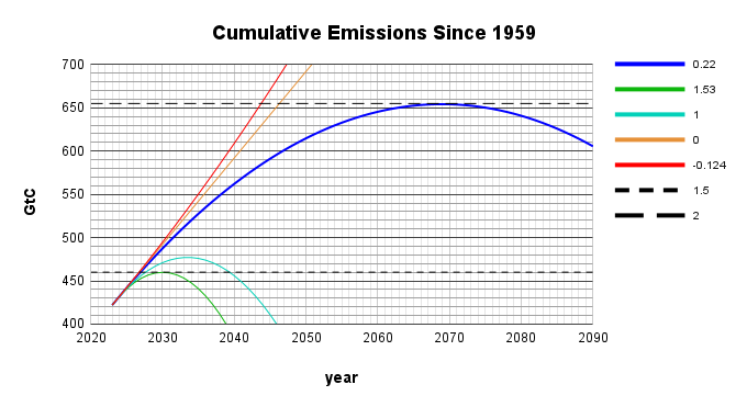
For \(x\)=1.53 GtC per year, we reach net zero in 2029 with cumulative emissions at about 455 ppm, as shown in the lowest curve, colored green and labeled "1.53". If we lower the value of \(x\) to 1 GtC per year, we reach net zero in 2034 with cumulative emissions above the 460 threshold but below the 655 threshold, as was already seen in part (d). Lowering the value of \(x\) still further to 0.22 GtC per year, we reach net zero in 2069 with a value of cumulative emissions at about 655 GtC, as seen in the blue curve labeled "0.22".

We can include two other curves for comparison. The orange line labeled "0" is the case \(x\)=0, where we hold the annual emissions to a 2024 value of 10 GtC per year. This is the scenario examined in part (b), where we reach 460 ppm in 2027 and 655 GtC in 2047. The red curve, labeled "-0.124" is the "business as usual" case, where we continue the 21st century trend of increasing the annual emissions by 124 megatonnes of carbon per year. In this last case, we pass the 460 threshold in 2027 and the 655 threshold in 2043.