Math 3118, section 4
Spring 2001
Some facts about the normal curve

Purpose: A bit of further explanation about the normal curve and how to work with it.
 

As explained in the text, the normal curve is given by the following equation:

We don't have to work directly with this function very often, so we'll just need to know about a few of its basic properties By one of the class exercises, 11.4.2:

• the values of the function are all  > 0.
• the graph of this function is symmetric about the y-axis;
  thus  f(x) = f(-x)  for all  x.
• the value of  f(x)  becomes very small when  x  grows very large.

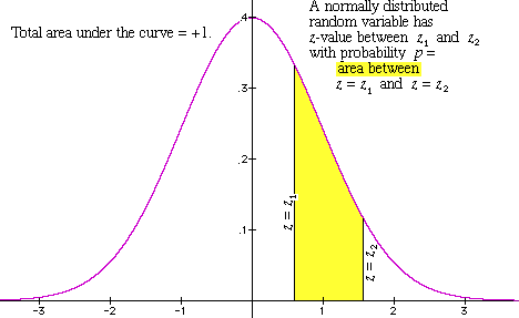
The graph of the function is shown in Figure 1 below.

Figure 1: the normal curve
 

By definition, a random variable is normally distributed if its probability distribution looks like the normal curve, suitably shifted and re-scaled. Thus:

• the curve is shifted so that its midpoint corresponds to the mean of our random variable,
• it is stretched so that 1 unit of distance from the standard normal curve corresponds to the standard deviation of our random variable, and
• the vertical scale is adjusted so that the total area remains equal to 1.
   

We don't have to work directly with the equation here!! Instead, we just have use Table 11.6 in chapter 11 of the text (on page 254 in the July 17, 2001 version) to find the area under the curve between the two corresponding  z-values. So, in Figure 1 above, the area of the yellow shaded region has to be  A(z₂) - A(z₁).  This area (being a number between  0  and  1)  tells us the percentage of our probability distribution -- or population -- for which the value of the random variable is within the indicated range. We'll explain below how to do this in some frequently encountered cases.

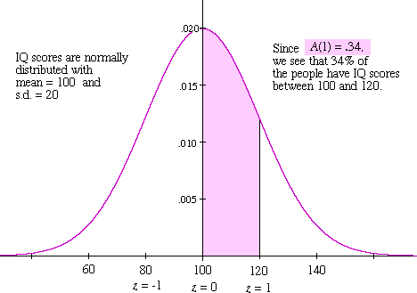
A couple of instances.In §11.5, we'll see that the outcome of an independent trials process -- repeated a large number of times -- is approximately normally distributed. IQ scores provide another example, as shown in figure 2 below.

Figure 2: the distribution of IQ scores
 

This example illustrates the fact that the re-scaling is "almost invisible". Namely, standard deviation is 20, so the difference between 120 and the mean ( = 100) is exactly  1  standard deviation unit. Therefore the area -- shaded in magenta in Figure 2 -- between the corresponding  z-values  (z = 0  and  z = 1)  is  A(1) = 0.34.  Hence, 34% of the population has IQ scores in this range.
 
 

Working with normal distributions

Part I:Determining the percentage of the population when a range of scores is given

1. Finding the area to the right of a given [positive] z-value.   For instance, this is the situation if we're given some test score above the mean and we want to find what percentage of the people taking the test had scores above that level.
    
   For a specific numerical instance, suppose that in a test with a mean of 73 and a standard deviation of 6, we want to know how what percentage of the students had scores of 80 or above. (This is like the discussion at the bottom of page 253 or the text.) So there are 3 steps:
   1. Find the  z-value. We work with 79.5 instead of 80; subtract the mean from this value, and then divide by the standard deviation:
               z = = = 1.083.
       
   2. Look up the value of  A(z)  in the table. We round off to  z = 1.1  and then look up:
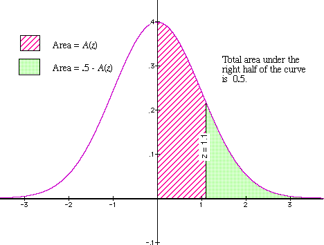
               A(1.1) = 0.3643.
      This gives the area that's shaded with red stripes in the diagram.
       
   3. Subtract from  0.5  to find the area of the right-hand tail of the distribution. Thus:
               0.5 - A(1.1) = 0.5 - 0.3643 = 0.1357.
      This area is shaded with green in the diagram.
   
   Thus, about 13.6%   of the students have scores of 80 or above.
    
   Figure 3: A(z) and the area of the "tail"
    
2. Finding the area within a given distance of the mean.   Given our information about IQ scores, suppose we want to know what percentage of the people have IQ score between 75 and 125, inclusive. Assuming that our scores just take integer values, we work with 125.5 and 74.5 when finding the corresponding  z-values.
   1. For a score of 125.5, we obtain:
               z = = = 1.275.
       
      For a score of 76.5, a similar calculation gives  z = -1.275.
       
   2. Working with the positive value, we round off to  z = 1.3   and look in the table to find:
               A(1.3) = 0.4032.
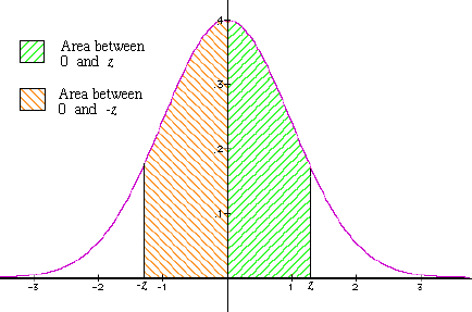
      This gives the area that's shaded with green stripes in Figure 4.
       
   3. By the symmetry of the graph, the area on the other side (with orange stripes) also has area = 0.4032. [Note that the z-value on the other side is exactly the negative of the one that we just looked at.] So, the total shaded area is:
               0.4032 + 0.4032 = 0.8064.
   
   Thus, about 80.6% of the people have IQ scores between 75 and 125, inclusive.
    
   Figure 4: The region within a given distance of the mean
    
3. Finding the area to the left of a given [positive] z-value.  Once again, we'll illustrate this with a specific example. So, let's suppose that 1000 students have taken an exam, where 100 points is the maximum score, the mean is 73, and the standard deviation is 5. We'll ask how many students had scores of 80 or lower.
   1. To find the z-value, we work with 80.5, since this "splits the difference" between 80 and 81. Here is our calculation:
               z = = = 1.5.
       
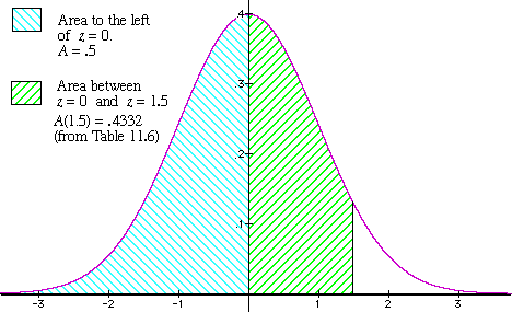
   2. As usual, we look in Table 11.6 to find  A(z):
               A(1.5) = 0.4332.
      This gives the area that's shaded with green stripes in Figure 5, corresponding to scores which are
      above the mean but below the indicated z-value.
       
   3. To find the total shaded area, we have to add the area to the left of the midpoint -- shaded in turquoise in Figure 5. Since it's exactly half of the entire area under the normal curve, this area is = 0.5. Hence, the total shaded area is:
               0.5 + 0.4332 = .9332.
       
   
   We conclude that 933 of the 1000 students had test scores of 80 or lower.

    

   
   Figure 5: The area to the left of a given positive z-value
    

Part II:Determining the range of scores when a percentage of the population is given

Each of these problems is "inverse" to the corresponding problem in Part I. Thus, in Part 1 we were given a range of scores and wanted to find the percentage of the population whose scores are in that range. In terms of Table 11.6, this meant that we calculated  z  and then looked up  A(z).  Here; the situation is turned around. We're given a percentage of the population, and we want to find what range of scores corresponds to it. So, we start by figuring out a value for  A(z)  and then looking in the table to find the value of  z  which corresponds most closely to it.
 

1. Finding the [positive] z-value such that a given percentage of the area under the normal curve lies to the right of that value.   (This question makes sense only if the given percentage is < 50%.)
    
   This is inverse to the problem discussed in Part IA, so that you can refer to the same figure. In Part IA we were given the  z-value, so we looked up the value of A(z) and then subtracted it from 0.5 to get the area of the tail -- shown with the light green [solid] shading in the figure. Here, we are given the area of the tail, so we do the steps in the opposite order, namely:
   1. Subtract from 0.5 to get the area under the normal curve between the midpoint (z = 0) and the horizontal line corresponding to the [still unknown]  z-value. This number is the value of  A(z)  that we have to work with.
   2. We now "read the table backwards" to find the sought-for  z-value. Thus, we look in the right-hand column of Table 11.6 to find the number that's closest to the value of  A(z)  that we just calculated. Our  z-value is on the same line in the left-hand column of the table. For better accuracy, if our value of  A(z)  is about halfway between two entries in the right hand column of table 11.6, then we can split the difference between the two corresponding  z-values.
       
      An instance: Let's determine the  z-value such that 10% of the population has scores above that value. This means that we have to take  A(z) = .5 - .1 = .4. Looking in the table, the closest value is  A(z) = .4032,  and this corresponds to  z = 1.3. In an applied problem, we still have to re-scale and shift. For instance in the case of IQ scores, with  mean = 100  and  s.d. = 20,  a  z-value of 1.3 corresponds to an IQ score which is  1.3·20 = 26  points above the mean, and thus to a score of  100 + 26 = 126.
       
2. Finding the [positive] z-value such that a given percentage of the area under the normal curve lies within  z  standard deviation units of the mean.
     This is inverse to the problem discussed in Part IB, so that you can refer to the same figure. In Part IB we were given the  z-value, so we looked up the value of A(z) and then multiplied it 2 to get the area under the the middle part of the bell curve -- shown as the total of the two shaded areas in the figure. Here, we are given the area of the symmetric middle part, so that we have to reverse the order of the steps and appropriately substitute division for multiplication. Thus:
   1. Divide the given symmetric area by 2, in order to find the value of  A(z).
   2. Look for this value in the right-hand column of Table 11.6. Our answer is then the  z-value on the same line of the table. For instance, suppose that we want to determine the IQ scores that characterize the middle  ² / ₃  of the population. Then we take  A(z) = ¹ / ₃  ( = ² / ₃ . ¹ / ₂ ). Looking in the table, the two closest values are  0.3159  and  0.3413.  These correspond to  z = 0.9  and  z = 1.0  respectively. Accordingly, our answer is about halfway between and thus corresponds to  z = 0.95. The actual range is between 19 points  ( = 0.95·20) below the mean and 19 points above the mean, i.e., IQ scores between 81 and 119.
   
    
3. Finding the [positive] z-value such that a given percentage of the area under the normal curve lies to the left of that value.   (This question makes sense only if the given percentage is > 50%.)
    
   Look at the figure in Part IC to help with understanding this case. We have to subtract 0.5 from our given area in order to find the value of  A(z)  to work with. For instance, if we want to find the score corresponding to the 85^th percetile, then we take  A(z) = 0.85 - 0.5 = 0.35. (Etc., by analogy with the other cases ... )

Back to the class homepage