The Mathematics of Satellite Images
Jonathan Rogness
University of Minnesota
What is a Satellite Image?
Satellites have sensors which respond to light power.
- Increased Light ⇒ Increased Voltage
- Analog voltage converted to a digital number (DN)
- Typical scales: 0-255 or 0-1023
Different sensors respond to different wavelengths on the Electromagnetic Radiation (EMR) Spectrum
EMR Spectrum
|
LandSat
- MSS: 4 sensors
- TM: 7 sensors
AVHRR
|
Spatial Resolutions
The spatial resolution of a sensor is the size of the smallest detectable feature.
- LandSat MSS: ~ 80m
- LandSat TM: ~ 30m
- AVHRR: 1km
LandSat: images have more detail, but the data sets are huge. Coverage only repeats every 18 days.
AVHRR: images can have daily coverage and are more reasonable for large projects, but can't detect small features.
From DNs to Images
Any single band can be displayed as a grayscale image, where 0 is black and 255 is White.
Otherwise we create "color composite" images.
True Color Composites
|
| Band | Displayed As |
|---|
|
|
| Red | Red |
| Green | Green |
| Blue | Blue |
|
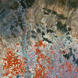
False Color Composites
|
| Band | Displayed As |
|---|
|
|
| NIR | Red |
| Red | Green |
| Green | Blue |
|
Introduction to Applications
Let's give a short description of three
applications:
- Vegetation Mapping and Monitoring
- Land Cover Classification
- Fire Detection and Prevention
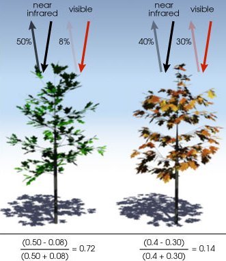
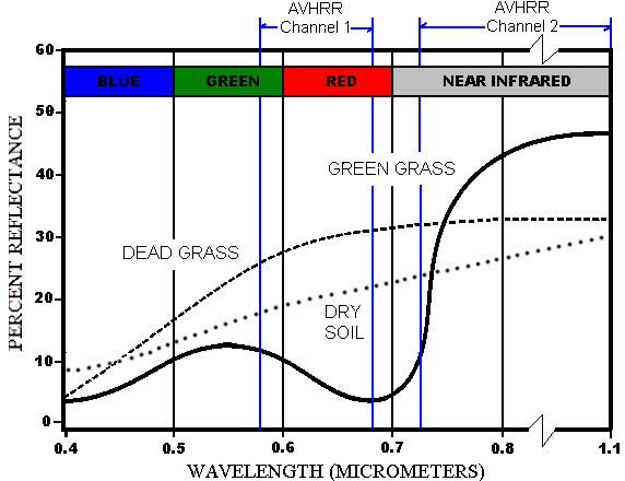
Vegetation
Healthy vegetation tends to absorb visible red light (AVHRR Ch1) but reflect NIR (AVHRR Ch 2). This leads to NDVI:
| N | ormalized |
| D | ifference in |
| V | egetation |
| I | ndex |
Definition. NDVI of a pixel = (NIR - Red) / (NIR + Red).
Minnesota NDVI, June 1992

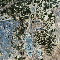
Land Cover Classification
This has been done globally on a 1km scale with AVHRR data, and a 30m scale in the US with LandSat TM data. There are two ways to classify pixels, supervised and unsupervised.
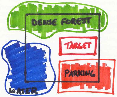
Supervised Classification
Idea: use previous knowledge to help the computer recognize certain spectral signatures.
Difficulties in Supervising
This isn't as easy as it sounds. Land cover is rarely consistent within one pixel, particularly for larger spatial resolutions. You need a very large database of nearly endless possibilities.
Unsupervised Classification
Idea: use a clustering algorithm to group similar pixels together. This is done without regard to pixel location; only spectral signatures matter.
| Pixel # | Ch 1 | Ch 2 | Ch 3 | Ch 4 |
|---|
| 1 | 99 | 122 | 140 | 150 |
| 2 | 101 | 120 | 143 | 152 |
| 3 | 160 | 165 | 180 | 181 |
Note that each pixel is a point in a n-dimensional space. For example,
P1 = (99, 122, 140, 150) in R4
Unsupervised Mathematics
There are various approaches:
- Try to determine in one pass which are closest to each other.
- Iterative Algorithms
- Principal Components Analysis (PCA)
Afterwards the computer gives us a LC map with each pixel colored according to its grouping. With prior knowledge (or ground observation) we can name each group.
Fire Detection and Prevention
This is a special case of the other two applications. Fires and smoke have fairly distinct spectral signatures. Also, current NDVI can be compared to previous years to gauge drought conditions.
Environmental Monitoring
Using vegetation indices and land cover classifications allows us to monitor ecosystem development, urban growth, deforestation, natural disasters, and more.
Highly recommended: http://earthshots.usgs.gov.
Potential Problems
Now let's consider three potential problems that arise when working with images.
- Sensor Calibration
- Image Registration
- Cloud Cover
Sensor Calibration
Design specifications don't survive the trip into space. How do we know much light power does each DN (0-255) represent? How does it change over time?
After each reading, sensors take another reading while looking into deep space. This is the base level for "absolute darkness" -- often a DN as high as 40!
The rest of the data must be scaled using this new minimum. (But what's the maximum?)
	true = 255 * (raw - 40)/("observed max"-40)
OR	true = C   * (raw - 40) for some C.
Scaled vs. Unscaled
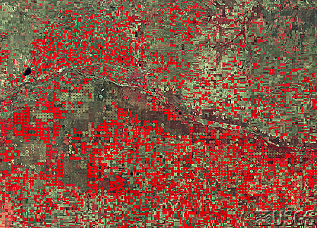

Image Registration
Monitoring specific sites requires annual / monthly / weekly / daily images. Time lapse comparisons of one pixel are hard, because the location is never quite the same. If you watch a slideshow of the "same" AVHRR images over time, a lake will jump around as much as 10km!
A common solution uses a Fast Fourier Transforms (F) and an Inverse Fast Fourier Transform (I).
Registration Process
- Choose a control image with a clear, distinct feature (e.g. a lake).
- Correlate every other image to the control image:
- Choose a window in the other image which includes the lake
- Find the maximum value of I(F(control) * F(window)).
- This shows you the offset, i.e. how to translate your image to match the control image.
Composites
Another approach: Composite Images. (10 Day composites are common.)
- Get multiple images of the same location
- At each pixel, use the values from the day with the highest NDVI values.
(Not just the highest values. For example, the highest values in Ch1 probably represent cloud.)
Problem: significant greenup can occur in 10 days!
Related issue: creating a mosaic of images.
Cloud Detection
Harder than you'd think!
There are too many cloud types to reliably recognize every "cloud spectral signature;" Besides, we can't do LCC for every pixel ever beamed down. We need fast run-time cloud detection techniques.
We tend to use quick "threshold tests." If a pixel fails, say, 3 out of 5 tests, we say it's a cloud.
CLouds from AVhRr (CLAVR)
Includes tests like:
- RGC: is Ch1 > 44% ?
- RR: is 0.9 < (Ch2/Ch1) < 1.1 ?
- TGC: is "temperature" < 249K ?
Cloud edges are hard to detect, so CLAVR is often done on a 2x2 grid.
- 0 pixels cloud: all 4 "clear"
- 1-3 pixels cloud: all 4 "mixed"
- 4 pixels cloud: all 4 "cloud"
CLAVR Results