Solutions to Homework 6
Math 5251 Fall 2006
Rogness

Unlike some of the previous materials I posted, I wrote these solutions out in Mathematica.  For convenience (mine) I didn't delete the Mathematica commands before posting this document online, but you should certainly feel free to ignore the bold-faced commands and just pay attention to the answers.

As always, these solutions aren't meant to be comprehensive, so let me know if you still have a question or spot a typo.  Thanks!

12.17

12.A

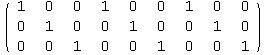
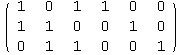
We know the Hamming [7,4] code is generated by the matrix

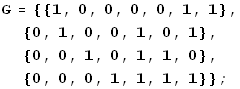
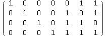
This is in "standard form," G = [ I | A ], so we know that the generating matrix for   is given by = [ - | I ].  More often we called this matrix H, because it's also the check matrix for the Hamming code.  See pages 223-224.

The dual code is a [7,3] code, and its codewords are all of the linear combinations of the rows of H:

One way to find the minimum weight of a linear code is via the proposition on page 222: d is equal to the minimum weight of the (non-zero) words.  By looking at the codewords we see the minimum weight is 4, so this code can in fact correct a single error.

14.02

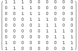
Here's the matrix:

There are a few ways to procede.  The first approach uses linear algebra by finding the row-reduced verion of the matrix.

We see that the resulting matrix has 7 non-zero rows, which means the dimension of the rowspace is 7.  However, I still have to find a generating polynomial, so this approach only gets me halfway.

The other approach is to notice that the polynomial b(x) used to generate the matrix is

Now we can find the "best" generating polynomial, which is the GCD of b(x) and -1; since we have a 9x9 matrix, n=9:

(Aha!  So b(x) must already divide -1.)  Now we can write down a "true" generating matrix for the code, by cycling the vector corresponding to b until its last 1 reaches the last column.

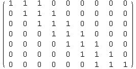
This is a 7x9 matrix, so the code must be a [9,7] code and have dimension 7.

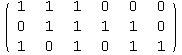
14.04

Roughly following the approach in 14.02, we have

We can immediately replace b(x) with a polynomial which divides -1 and generates the same code:

As a 9-dimensional vector, that's 100100000, so the generating matrix is

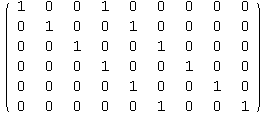
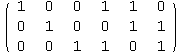
That's a 6x9 matrix, so C is a [9,6] code.  To find a check matrix we can procede as in 12.A, or we can use the special form of a check matrix for cyclic codes, as described on page 236:

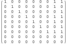
So the check matrix is

We can verify that all the rows of G are orthogonal to the rows of H by computing the following matrix multiplication;

(This works because each entry in that product comes from a dot product with a row of G with a column of , and the columns of are the rows of H.)

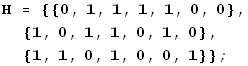
14.B

Because the rows of G are linearly independent (which you can see by inspection, or by row reduction, as we'll show in a second), this is a true generating matrix of size 3x6, so it generates a [6,3] code.

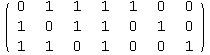
The standard form of the matrix can be found as follows.  I'll call this matrix G2.

This is in the form [ I A ], so the check matrix is [ - I ] and will have size (n-k)x n = 3x6.

By inspection, none of the columns in H are the same, and they're all nonzero.  Hence by the theorem on p234 (and the special-case corollary on p235), the minimum distance is at least 3 and it can correct at least one error.  In fact that's all that it can correct, because there are three columns which are linearly dependent.  (For example, the first three columsn added together give 0.)  So the minimum distance is exactly 3.

The syndrome corresponding to 0 transmission errors should always be 0:

The syndromes for single digit errors are calculated by e :

To decode the first word:

So the error vector is 001000 and the corrected word is

The syndrome for the second word is

Which corresponds to an error in the second bit, so the corrected word is 100110.

17.06

In class I called this type of matrix "Vandermonde (1st Version)," and you can find its determinant using the amazing theorem on page 278.  Here's the correct answer (Mathematica is just doing number crunching here, nothing amazing):

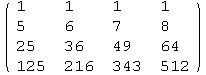
Created by Mathematica  (December 16, 2006)