Mathlets

Introduction

Quick Links

A mathlet is a generic term for a small, interactive, platform-independent tool for teaching math. Gene Klotz tells me that the term was coined by June Lester. Over the past few years I've developed a lot of these materials, and they've been scattered across multiple course webpages. This page is an attempt to create a single, organized list of mathlets for other people to use in their classes. The materials here are roughly organized by course, but there's a lot of overlap; parametric curves might be covered in PreCalculus, single- and multi-variable calculus courses, for example. You might also be interested in the following pages:

These mathlets were created using LiveGraphics3D, a Java applet by Martin Kraus. If you'd like to make similar materials, you can read an article Martin and I wrote about how to create mathlets using LiveGraphics3D.

A Note for Instructors: some links below are for long modules with many mathlets and lots of accompanying text. Other pages have a single picture with no accompanying text -- this is common when I just want to show a picture in class and will explain what we're looking at. If you'd like me to add any text to a page, please let me know. I've also included an indicator of how ready each mathlet is for general use:

		These mathlets are in good shape.
		These applets need improvement, either with the text or graphics, as time permits.
		These are usable, but just barely. In some cases I have a good idea but I just don't like the implementation. I'm always open for suggestions on how to improve these.

Directions for Using these Mathlets

In some web browsers, the mathlets will become active once you move the mouse pointer over the picture; in others, you might need to click on the picture first. Once active, you can use the following controls:

Click+Drag: rotate the image (for 3D images only)
Shift+Click+Drag Up/Down: zoom in/out
Home: reset the image
Double Click: stop/restart the animation (if applicable)
's' key: cycle through normal mode, parallel stereo mode, and cross-fusion stereo modes.

Many of the mathlets allow you to click and drag points with the left mouse button to adjust variable values.

PreCalculus (Broadly Construed...)

	Animated Proof of Pythagorean Theorem
	Circle of Radius 5. Click and drag on the point.
	Examples of Intersecting, Parallel, and Skew Lines in 3D.

Single Variable Calculus

Continuity and Differentiability

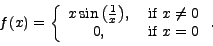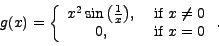	is continuous, not differentiable at x=0
	is continuous and differentiable at x=0

Computing Volumes using Integrals

	Surface and Solid of Revolution (Basic) Surface of Revolution. Shows the resulting surface when the graph of y = x ² is rotated about the x-axis. Volume of a Solid of Revolution. This shows the cross sections of the solid bounded by the surface in the previous mathlet. It's hard to spot, but there's a black point where the cross section touches the original graph of y = x ²; you can click and drag the point to move the cross section.
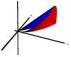
	Surface and Solid of Revolution (Advanced) Surface of Revolution. Shows the result of rotating the region bounded by y = x ² and y = x about the x-axis. Volume of a Solid of Revolution. This shows the cross sections of the solid bounded by the surface in the previous mathlet. Click and drag the black point to move the cross section. The current value of x and the approximate area of the cross section is shown below. There is also an animated version of this mathlet in which the cross section automatically slides back and forth.
	Volume of a Pyramid using Cross Sections View the cross sections of a pyramid of height 3 with a square base of area 4. Click and drag any of the black points to move the cross section. The current value of x and the approximate area of the cross section is shown below. There is also an animated version of this mathlet in which the cross section automatically slides back and forth.

Taylor's Theorem

Taylor Approximations of the Square Root Function. This shows the n^th-degree Taylor polynomials of the function f(x) = sqrt(x), centered at x=a, for n=1, 2, 3, 10. Click and drag on the point to adjust the value of a.

Multivariable Calculus and Vector Analysis

Surfaces, Cross Sections and Level Curves

	Interactive Gallery of Quadric Surfaces. This is a collection of mathlets which lets students interactively investigate the cross sections of quadric surfaces. Students can also adjust the values of the constants in the equations of the quadric surfaces to see how they affect the shape of the surfaces. 2005 version on JOMA Current version on www.math.umn.edu
	Slicing a Paraboloid A cross section of a surface is really the intersection of the surface with a plane, but teachers will often talk about "slicing" or "chopping" a surface with a big knife along the plane. This animation shows the elliptical paraboloid z = x² + y² being sliced along a plane z = k.
	Contours of a Saddle This animation shows horizontal planes moving through the saddle z = x² - y², leaving a "trail" of cross sections as it goes. These cross sections then move to the xy-plane, forming the contour map (i.e. a collection of "level curves") for the surface.
	"Nonstandard" cross sections of a saddle Typically we look at cross sections defined by x = k, y = k, z = k, or (in the case of the directional derivative), ax +by = k. This animation shows the saddle z = x² - y² and its intersections with the planes x = a z. Here's an interesting challenge problem: are the cross sections really hyperbolas, or do they just look like it?

Parametric Curves and Surfaces

	Particles in Motion: Parametric Curves with Velocity Vectors (This page contains a number of applets and takes a while to load.)
	2D Curvature Examples. Watch a particle move a long a curve along with the unit tangent vector, unit normal vector, and osculating circle: parabola; cubic; quartic; cusp; all (large file)
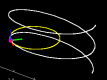
	3D Curvature Examples: Watch particles move along three-dimensional curves, including the TNB (Frenet) Frame and the osculating circle: helix; elliptical helix; tornado; exponential spiral; twisted cubic; all (large file)
	Parametrized Surface: A Torus
	Is the cone a smooth surface or not? Watch this animation of the normal vector r_u×r_v on the cone and decide!
	Continuously Varying Normal Vectors on a Paraboloid

Derivatives

	Geometric Interpretation of Partial Derivatives
	Directional Derivative Example
	Tangent Plane with Vectors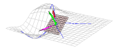
	A function with a partial derivative which does not exist.
	A function with partial derivatives which is not differentiable.
	A differentiable function with discontinuous partial derivatives.
	Lagrange Multipliers; this has no accompanying text, but if you know how Lagrange multipliers work you can probably figure out the images!

Integrals and Integration Theorems

	Estimating Double Integrals
	Change of Variables: Polar to Rectangular Coordinates
	Change of Variables: A Nonlinear Transformation
	Stokes Theorem: infinitely many surfaces with the same boundary
	Stokes Theorem: infinitely many surfaces with the same boundary (different classroom version)
	Stokes Theorem: surfaces with a vector field G=curl(F): the flux across all of these surfaces is the same!

Topology and Geometry

	Costa Surface. This surface can be constructed it with eight pieces. Each piece is a rotation and/or reflection of the fundamental piece. You can also view an animation showing how they fit together.
	Gluing a rectangle into a torus (donut) using the standard two-stage process First wrap the rectangle into a cylinder, and then glue the two ends of the cylinder together to form the torus.
	Gluing a rectangle into a torus in a single stage For topologists: this demonstrates how to visualize the single 2-cell in the "minimalist" CW-decomposition of the torus.
	Standard Immersion of a Klein Bottle
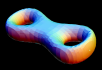
	Double Torus (aka Two-Holed Torus, Dogtoy Surface...)
	Deformation of a cube into a sphere
	Deformation of a punctured sphere into a plane. You might also be interested in the image of a spherical triangle under this deformation. Be careful about any generalizations, however; the result depends on which triangle you use.
	Deformation of the Earth into a plane. Mathematically this is the same as the previous applet, but the sphere has outlines of Earth's continents. Notice that the equator never changes during the deformation. Also pay attention to Antarctica, which includes the South Pole, and Greenland, which is close to the north pole. Thanks to Martin Kraus for creating the polyline outlines of the continents using coordinates from Mathematica's `WorldData` package.

This page is http://www.math.umn.edu/~rogness/mathlets.shtml and belongs to rogness@math.umn.edu The views and opinions expressed in this page are strictly those of the page author. The contents of this page have not been reviewed or approved by the University of Minnesota.

Many thanks to css/edge for a lot of the ideas used in the creation of this page.

[an error occurred while processing this directive]